XGSLab™ Grounding System Analysis Assumptions
GSA and GSA_FD Modules
The following table summarizes the main assumptions on which GSA and GSA_FD module are based.
| Aspects Considered | GSA | GSA_FD |
|---|---|---|
| Resistive coupling | Yes | Yes |
| Capacitive coupling | No | Yes |
| Self impedance | No | Yes |
| Mutual impedance | No | Yes |
| Soil parameters | ρ | ρ, ε = f(ω) |
| Propagation law | 1/r | e-ϒr/r |
The following graph represents the application domain of the two modules. The highlighted area indicates the usual conditions at power frequency.
The graph is obtained by a parametric analysis with a square meshed test grid energized with a current injected in a corner and made of copper. The analyzed parameters were grid size “D,” soil resistivity “ρ” and frequency “f.” In its application dominion, the errors made by GSA in the GPR and touch voltages calculations are lower than 10%.
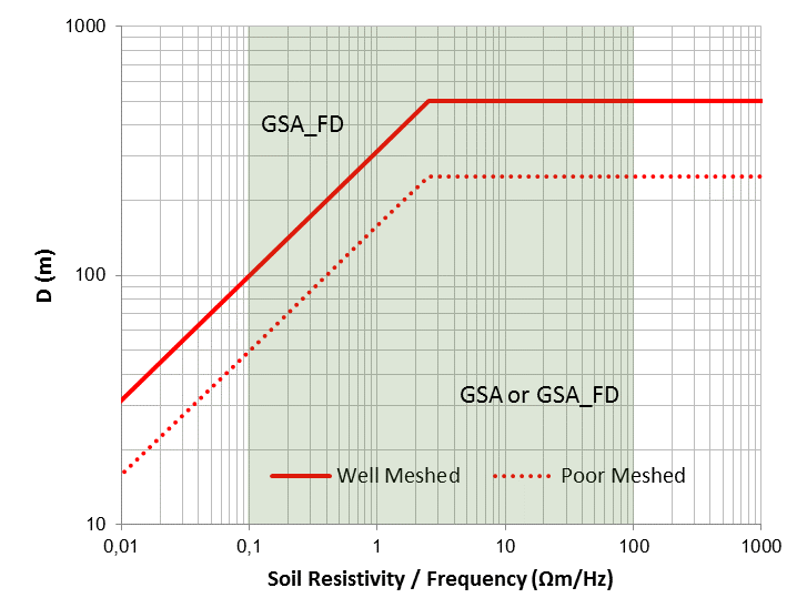
Application domain of GSA and GSA_FD
In practice, in case of well-meshed grids, application limits of GSA can be defined as a function of the wavelength of the electromagnetic field in the earth as follows:
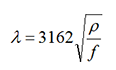
where λ (m) = wavelength, ρ (Ωm) = soil resistivity and f (Hz) = frequency.
The previous diagram indicates that GSA can be used if “D < λ/10”. GSA also requires “D < 500 m” as reasonable limit.
The application limits will be lower if the grid shape is not regular, if the meshes are sparse and if the grid is made of steel or other high resistivity metal. In all these cases, the limit related to poor-meshed grids as defined by the red dashed line should be considered.
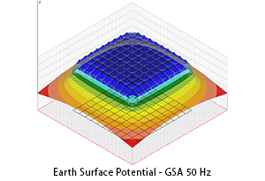
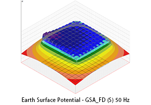
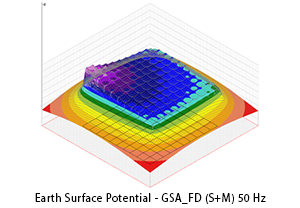
The following three figures show the earth surface potential distribution calculated by applying GSA and GSA_FD to a 100 m x 100 m grid with the same injected current, the same frequency (50 Hz), the same injection point (marked with arrow) and the same soil model.
The qualitative difference between results is evident. GPR and impedance to earth tend to grow whether self impedance and mutual impedance are taken into account. High frequency or low soil resistivity can make this difference even more evident.
Of course, a difference in the earth surface potential distribution corresponds to a difference in touch and step voltage distribution.
In brief, in grounding system analysis at power frequency, GSA can be used in many practical situations but it tends to underestimate the results if the grid size is greater than one tenth of the wavelength of the electromagnetic field, while GSA_FD may be applied in all conditions.
The answer is simple but not trivial. GSA requires an easier data entry, accept rough layouts and requires fewer computer resources.After these conclusions, a question could arise: Why not just use GSA_FD?
GSA_FD requires additional information about the topology of the conductors system and in order to calculate their self and mutual impedances and a well finished layout. Moreover GSA_FD requires more experience in the evaluation of results. If GSA cannot be used, GSA_FD is the right solution.
XGSA_FD and XGSA_TD Modules
XGSA_FD is based on the same model of GSA_FD but extended to overhead conductors. The application limits of XGSA_FD can be assumed from DC to about 100 MHz. XGSA_FD greatly expands the application field of XGS and makes it a real laboratory for engineering applications and for research. XGSA_FD is an irreplaceable tool when conductors are partly overhead and partly underground. This situation is usual in electromagnetic fields evaluation (where sources may be underground cables or overhead wires) or interferences analysis (where often the inductor is overhead and the induced is underground). Anyway XGSA_FD operates to a single frequency.
XGSA_TD can calculates the response in the time domain of a conductors network energized with a current or voltage transient.
As known, the methods to calculate the transient behaviour of conductors network in the time domain can be divided into two main categories: those based on the calculation of the solution directly in the time domain and those based on frequency domain calculations and then using the forward and inverse Fourier transforms.
Methods of the first category require low frequency and quasi-static approximations and in addition do not allow considering the frequency dependent characteristics of the grounding system.
Methods of the second category use an electromagnetic field approach for the calculation of the response of the grounding system in a wide range of frequencies and have a good accuracy because they are based strictly on the principles of electromagnetism. On the other hand, in these methods, a system of equations has to be solved for every particular frequency, and a large number of discrete frequency points over the frequency band are chosen to satisfy the frequency sampling theorem.
XGSA_TD is based on the second category methods and uses XGSA_FD as solver in the frequency domain. Then the application limits of XGSA_TD can be assumed as the same of XGSA_FD and in particular the maximum bandwidth of the input transient should be lower than 100 MHz.
This means that XGSA_TD can consider transient input as switching transients, standard lightning currents and also fault transients in GIS.
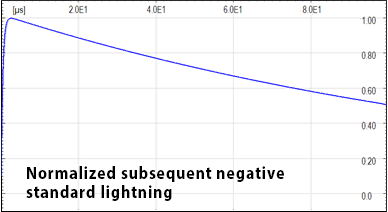
The simulation of lightning represents the most typical application of XGSA_TD. The lightning current can be simulated by using the standard short stroke wave form IEC 62305: first positive; first negative; subsequent negative.
With the direct Fourier transform, the time domain input transient is decomposed in the frequency domain.
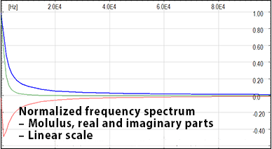
In the following figures the normalized wave shape of the subsequent negative standard lightning current and their normalized frequency spectrum. The spectrum can be neglected when normalized values are lower than about 10-3 - 104. The standard lightning bandwidth is lower than a few MHz also for the fastest lighting, the subsequent negative ones.

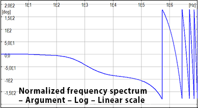
After the calculation in the frequency domain (taking into account a reduced number of critical frequencies to limit the calculation time), the response in the time domain is obtained with the inverse Fourier transform.Normalized frequency spectrum of subsequent negative standard lightning – Log-Log
The evaluation of lightning effects is important. For instance, current generated by a stroke flows in the LPS conductors and dissipates in the soil. The electric and magnetic field generated by such high voltages and currents may cause damage of equipment and may be dangerous for people.