XGSLab IEEE Standard 80 Benchmarks
IEEE Standard 80 provides guidance for safety related to the grounding in AC substations. This standard highlights the dangerous conditions that may occur during a ground fault that can severely or fatally injure individuals who are in contact with metallic objects or simply in the area. The Annex H of IEEE Std 80-2013 provides readers with examples to compare the calculation methods in the standard with several software tools. The results below are based on calculations using the GSA_FD, XGSA_FD, and NETS modules and demonstrate the high accuracy users can expect when performing studies in the software. The XGSLab software uses the Partial Equivalent Element Circuit (PEEC) Method, which combines circuit and electromagnetic theory into a single calculation and enables complex analyses.
The examples below are derived from IEEE Std 80-2013 Annex H. Refer to the standard for additional details.
Soil Analysis
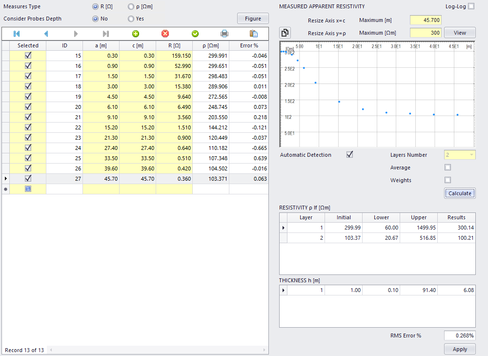
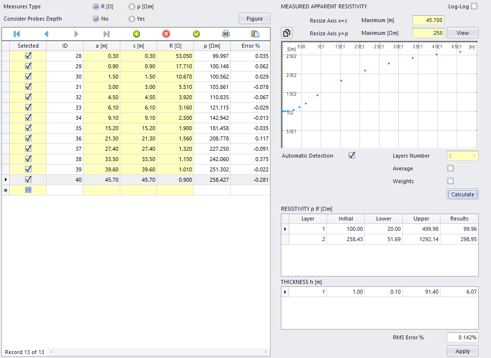
The IEEE Std 80 soil analysis benchmark provides two 4-pin (Wenner Method) measurement traverses for two soil systems. These measurements are mathematically derived due to the difficulties and errors that can occur when performing actual field measurements to determine the correct soil model. The table in IEEE Std 80 2013 does show inaccuracies, specifically for the shallower measurements, fortunately the mathematically derived measurements for identical soil models are available in IEEE Std 81 2012 Table 3. The first soil model is a two-layer where ρ1 = 300 Ω-m for 20 feet (6.096 m) and ρ2 = 100 Ω-m. The second soil model is a two-layer where ρ1 = 100 Ω-m for 20 feet (6.096 m) and ρ2 = 300 Ω-m. The XGSLab results based on the IEEE 81 mathematically derived measurements align very well with the soil models.
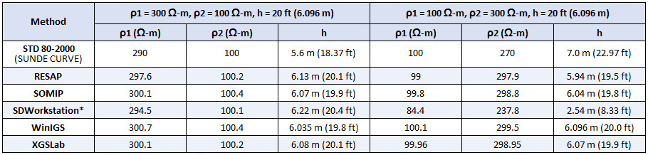
©2020 IEEE. Reprinted, with permission, from IEEE.
*Does not allow measurements below 1.77 ft spacing.
As XGSLab provides users many tools to resolve soil modeling challenges, the values as entered into the software are provided for ease of comparison. No adjustments are made to the Soil Resistivity Analyzer algorithm to arrive at the answers above, and each measurement as provided in IEEE Std 81 table are shown below:
Ground Grid 1 Analysis
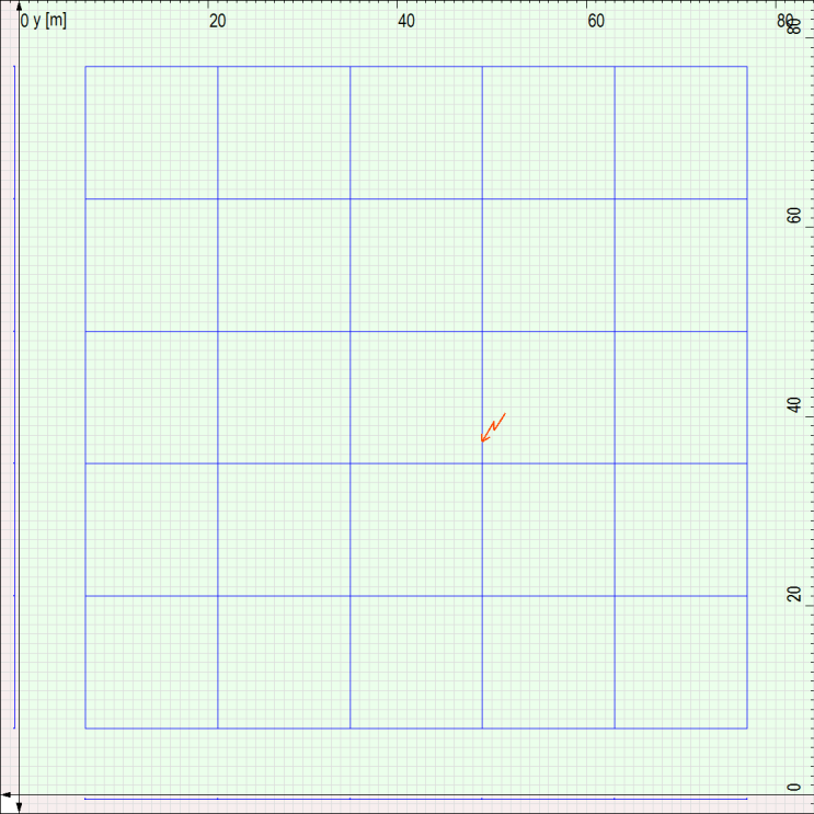
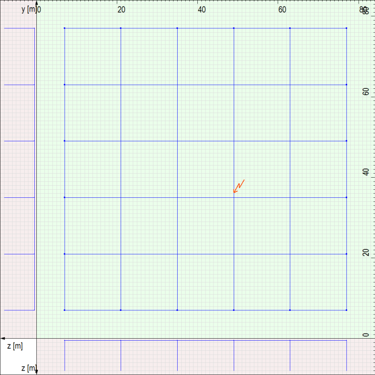
The first ground grid considered in the annex is a symmetrically spaced square grid without ground rods. As described in IEEE Std 80, the touch and step voltages above correspond to a specific location relative to the ground grid and a maximum voltage determined by the software. The ground grid consists of 2/0 copper buried at a depth of 0.5 m and modeled in a uniform soil model of 140 Ω-m, as shown below.
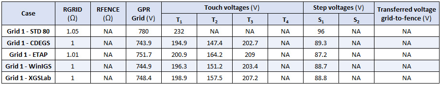
©2020 IEEE. Reprinted, with permission, from IEEE.
Ground Grid 2 Analysis
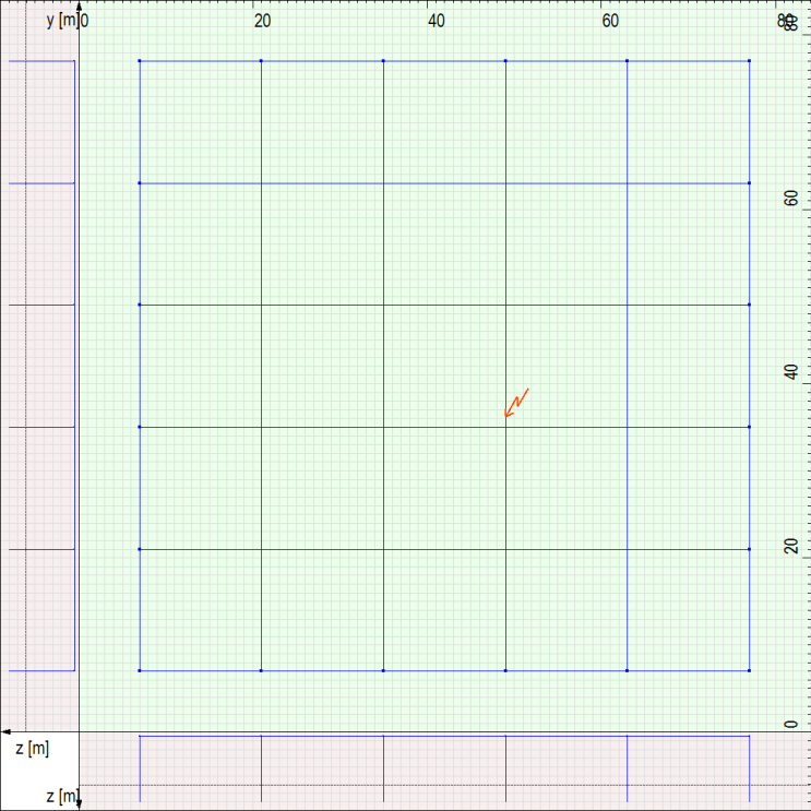
The second ground grid considered in the IEEE Std 80 annex is a symmetrically spaced square grid, which now includes ground rods along the perimeter. The ground grid consists of 2/0 copper buried at a depth of 0.5 m, with 7.5 m long ground rods, and is modeled in a uniform soil model of 140 Ω-m, as shown below.
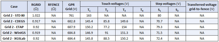
©2020 IEEE. Reprinted, with permission, from IEEE.
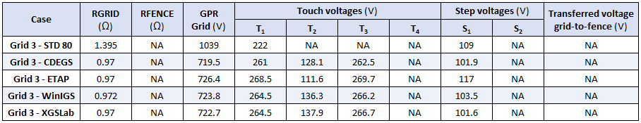
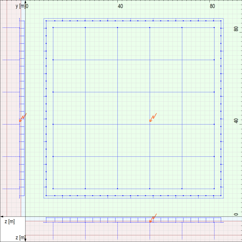
Ground Grid 3 Analysis
The third ground grid considered in the IEEE Std 80 annex is identical to Grid 2, but is now is a two-layer soil model where ρ1 = 300 Ω-m at h = 20 ft (6.096 m), and p2 = 100 Ω-m. The ground grid is shown below.
©2020 IEEE. Reprinted, with permission, from IEEE.
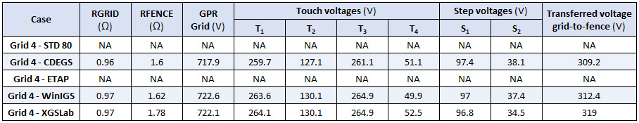
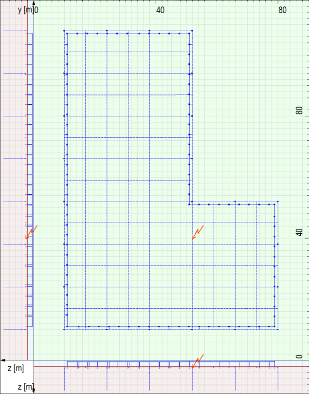
Ground Grid 4 Analysis
The fourth ground grid considered in the annex includes a separately grounded fence in the model. The calculation method provided by IEEE Std 80 and some software are not capable of assessing two independent electrodes in the same soil systems. As a result, this example is a comparison of a subset of the software. The fence is placed 3 m outside the grid perimeter with a fence conductor loop 4 m outside the grid perimeter. The annex does not state the frequency of the grounding connections from the fence conductor loop, and the XGSLab model assumes every third fence post was bonded to the fence conductor loop. The ground grid, fence, and fence conductor are shown below.
©2020 IEEE. Reprinted, with permission, from IEEE.
For this grid, T4 and S2 represent the voltage difference based on the fence and fence conductor loop. In a transferred voltage analysis, such as a separately grounded fence in grid 4, the transferred voltage typically is expressed as the GPR. In the IEEE Std 80 annex, the reported transferred voltage refers to the difference of the potential of the grid (722 V) and the fence (403 V), resulting in 319 V.
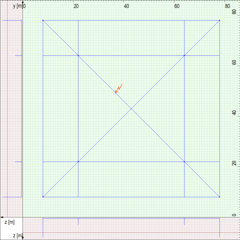
Ground Grid 5 Analysis
The fifth ground grid considered in the annex is an L-shaped grid with ground rods and a fence. The grid components are consistent with previous grids using 2/0 copper buried at a depth of 0.5 m, with 7.5 m long ground rods, and modeled in a two-layer soil model. The annex does not specify the frequency of grounding for the fence. The XGSLab model assumes every third fence post is bonded to the fence conductor loop. The modeled ground grid in XGSLab is shown below.
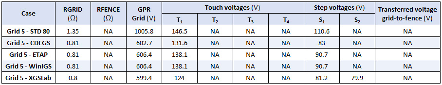
©2020 IEEE. Reprinted, with permission, from IEEE.
Unlike previous grids, T1 and S1 for grid 5 are calculated throughout the L-shaped grid with a spacing of 0.5 m and represent the maximum voltage. S2 is described as the voltage 1 m from the top left of the grid on a diagonal, but no results are provided from the other tools. Regardless the XGSLab results are provided as described in the standard.
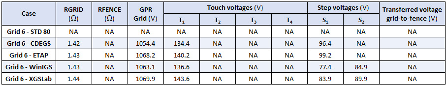
Ground Grid 6 Analysis
The sixth and last ground grid considered in IEEE Std 80 annex is a square grid with non-symmetrical spacing of the ground grid and varied ground rod lengths. Ground rods on the perimeter of the grid are modeled at a length of 7.5 m long, with the interior rods at a length of 2.5 m. The modeled ground grid in XGSLab is shown below.
©2020 IEEE. Reprinted, with permission, from IEEE.
In IEEE Std 80 Annex H, the description of step voltages S1 and S2 differ from the reference figure H.8. For the XGSLab values above, S1 is the difference in the earth surface potential along the diagonal of the upper-right corner of the grid matching the figure. The S2 is the worst-case step voltage within 1 m of the perimeter conductor using a 0.5 m difference in surface potentials. Note that the S2 is lower than the S1. S1, along the diagonal from the perimeter of the grid, captures a higher surface potential gradient than surface potentials developed on a 0.5 m surface potential gradient. This is important to note as tighter surface potential steps will produce more accurate results.
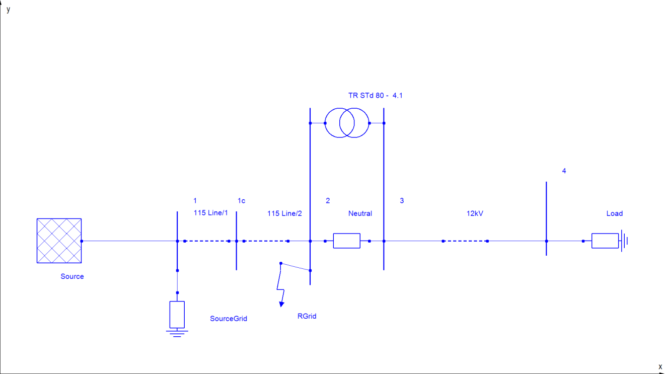
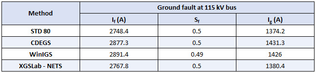
Fault Split
The ground current split for a distribution substation with a remote source is determined through the methods described in IEEE Std 80 and a subset of the software. This system consists of a remote source with a 10-mile long transmission line connected to a substation with a 1 Ω grid that feeds a 2.5 mile long distribution line and load. The system as modeled in XGSLab is shown below:
©2020 IEEE. Reprinted, with permission, from IEEE.
XGSLab™ Grounding Solution
XGSLab is one of the most powerful software for electromagnetic simulation for power, grounding and lightning protection systems and the only software on the market that takes into account International (IEC/TS 60479-1:2005), European (EN 50522:2010) and American (IEEE Std 80-2000 and IEEE Std 80-2013) Standards in grounding system analysis.