Soil Modeling and Soil Resistivity Interpretation

Soil modeling is an important step in the analysis of grounding systems as the soil affects the system impedance and the safety criteria used to assess grounding performance. Developing a soil model can be a simple task, given quality measurements and advanced tools, like Soil Resistivity Analyzer (SRA), to aid in interpretation of the measurements. Even with advanced tools, many measurements need more engineering judgment to make an adequate interpretation of the soil measurements. The goal is to develop an accurate soil model that provides an efficient grounding design to meet the tolerable voltage limits. This article focuses on the interpretation of soil resistivity measurements to determine a soil model and is a resource for engineers designing and analyzing grounding systems.

Soil Resistivity Data

As discussed in the Soil Resistivity and Field Testing article, those analyzing grounding systems are primarily concerned with the soil resistivity typically expressed in Ω-m. Soil resistivity measurements at several locations within the site, or as close as possible, are necessary due to the significant variation of resistivity. The most common methods for testing are the Wenner and Schlumberger methods, which measure an apparent resistance with multiple variations in the spacing of the test probes. The figure below shows the change in equipotential contours path as different resistivity layers are encountered.

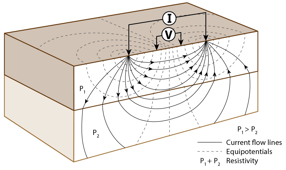
Soil resistivity measurement

Comparing the change in apparent resistance provides engineers a trend, indicating a uniform or multilayer soil resistivity model. Converting the apparent resistance to apparent resistivity, it can be easier to visualize that a set of measurements with a consistent resistivity would be accurately characterized with a uniform soil model. Far more common, the apparent resistivity increases or decreases at greater depths resulting in a multilayer soil model. As software allows hundreds of calculations to be evaluated quickly, the next section describes how SRA can be used to evaluate soil data to develop a soil model to evaluate a grounding system.

Developing Soil Models From Soil Resistivity Measurements

The real-world electrical characteristics of the soil are approximated in XGSLab with a soil model. The number of soil layers and resistivity of each layer is important to accurately characterize, but are often an area of challenge for many engineering projects. Understanding the soil modeling calculation methods supports better engineering decisions for interpreting measurements.

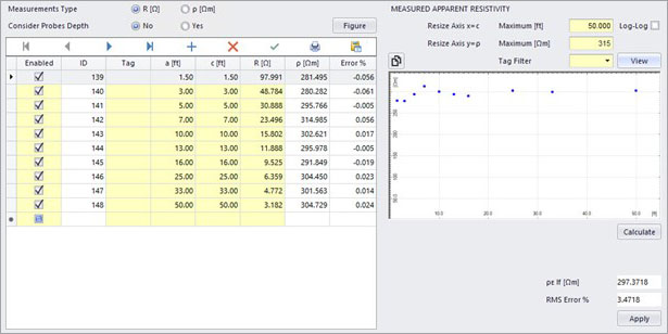
First is an example of a uniform soil model, as shown in the XGSLab SRA calculation below. The apparent resistivity for all measurements is approximately equivalent to 300 Ω-m, thus a uniform soil model would accurately represent this scenario.

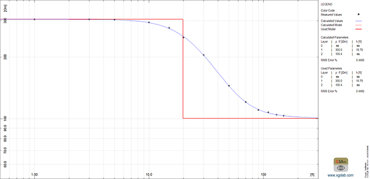
Uniform soil models are uncommon for utility scale grounding systems in many regions, as typical measurements show variation in the soil stratification requiring two, three, or more soil layers. Instead of the uniform resistivity, the table below represents a simple two-layer soil model. The resulting plot from SRA shows the steep downward slope as the resistivity changes from higher resistivity to lower resistivity.

Interpretation of measurements is possible by hand with two-layer models, and there are additional resources provided in standards and white papers to aid in converting measurements to approximate the top and bottom soil layers. Progressing to three or more layers in a soil model requires software tools to more accurately calculate and interpret the measurements. Accurately evaluating the grounding system performance with multilayer soil models is only possible with software like XGSLab.

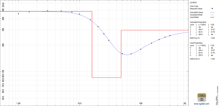
As shown below, the apparent resistivity of this three-layer begins at a higher resistivity of approximately 500 Ω-m before descending to a lower apparent resistivity. Instead of approaching a steady resistivity value, as observed in the two-layer model, there is an increase in apparent resistivity for longer traverses. This change in the slope indicates three layers, with a high to low to high resistivity relationship.

XGSLab SRA provides an additionally benefit in providing the RMS error, or the root mean square error, that indicates the deviation of calculated values from the measured values. This is a method to determine how well calculated values fit to the actual measurements. Forcing measurements corresponding to a three-layer model to a reduced two-layer model results in a significant increase in the RMS error % from 1.9% to 13.92%:

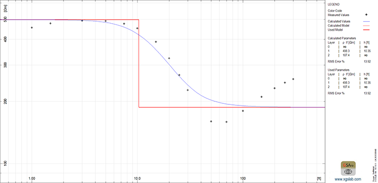
In this case the RMS error is an indication of an error, as a three-layer model reflects the soil resistivity stratification, but engineering judgement is required to determine an acceptable soil model. The acceptable level of RMS error is dependent upon the other data engineers may have before any final soil model is determined. Engineers should use the software tools to guide their interpretation, but not direct their decisions. This will be discussed in greater detail in the next section of this article.

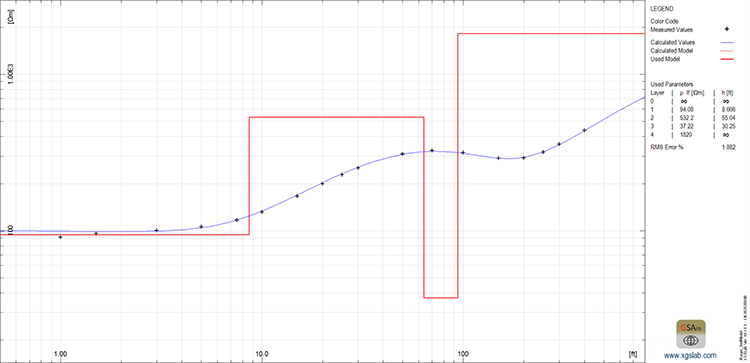
As more soil layers are encountered, the measurements will indicate a greater number of slope changes of the trend line. Encountering three changes in the slope is an indication of four-layer soil model as shown below.

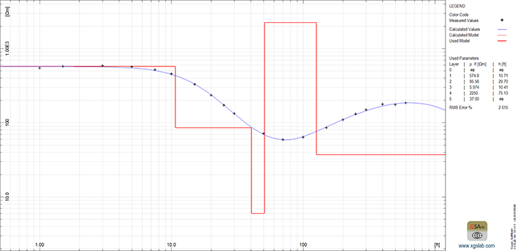
Similar to the example above, measurements encountering four changes in the slope is an indication of five-layer soil model. Where the slope change is clearly moving from a high resistivity to a lower resistivity, the slope is typically easier to visually affirm each layer of the soil model plot. If measurements reflect a low resistivity above an even lower resistivity layer, SRA is very helpful in finding and considering these increases in slope, as shown in the five-layer model below.

The typical number of soil layers is generally relative to a region and corresponding geology. Areas in the plains may be relatively consistent soil resistivity for hundreds of feet. Other regions, such as the mountain ranges, can see more dramatic changes in resistivity and corresponding increase in soil layers. Additionally, measurements to greater depths are more likely to face varying soil resistivity. Large grounding systems typical of higher voltage substations often require more soil layers, while small temporary substations may see one or two layers even in more stratified regions.

Soil Modeling Statistical Methods

Projects typically include multiple measurements at a site, providing engineers with multiple traverses to evaluate. From these measurements, an engineer must determine the best values to represent the soil electrical characteristics, often where there is some variance in the multiple traverses. Statistical approaches aid in the soil model development, such as the previously mentioned RMS % error.

The RMS error % is an indication in the variation that exists from the calculated soil model compared to the actual measured value. This can be useful in understanding if the measurements’ have significant variation, but can be dramatically increased where a single measurement is erroneous or out of trend with the other measured points. Lower RMS % error is affirmative to a soil model’s accuracy, but again more a reference tool for engineering decisions.

Providing weights to measurement points is another statistical method to prioritize certain values that have higher importance. For soil modeling, the shallower and deepest measurements have a significant effect on the performance of the grounding system. These layers often, but not always, have a greater effect on a grounding system impedance and safety criteria.

Most are familiar with averaging method, that is useful in taking a set of quantities and reducing the deviations. The benefit of averaging of soil modeling is dependent on the data and geographic sources. Averaging measurements from multiple sites with different geologic characteristics to determine a single soil model would be an obvious erroneous approach, as the grounding systems are affected by the local soil resistivity characteristics. Averaging multiple measurements in a single site can be acceptable in developing a final soil model. Reviewing each of the individual traverses is important, as the interpretation of measurements is looking at the trend of measurements to calculate a soil model. Taking perpendicular measurements, one traverse may be affected by some interference or errors, which would negatively impact the study if an engineer averaged errors or interference into measurements.

In addition to statistical approaches, splicing final soil models is another method for engineers to combine multiple measurements. This is a common technique where limitations provide only shallow measurements at the site of interest, while longer measurements are taken some reasonable distance away. Appending the bottom soil characteristics from the longer measurement to the shallow local soil model can give the most accurate soil model for a site.

Additional Resources to Consider

Interpreting soil resistivity measurements, it is important to understand some additional data to consider. First, most project will include soil borings at several locations of the project site. These can provide soil characteristics and as well as the location of any water table, typically boring tens of feet deep. These soil borings can be used to compare the soil characteristics of material to the resistivity measurements and resulting soil model. In some cities, counties, and states well drilling information is also publicly available and may provide data to depths of 100 feet or more.

As discussed in the soil resistivity field testing article, there are multiple challenges in obtaining quality data. When traverses do not align well with each other, it may be challenging to determine which values are accurate or affected by errors. An engineer responsible for the design and analysis of the grounding system can have better understanding of the site by participating in the soil resistivity measurements. Calculations can be performed on site to guide in-field changes to the scope of field testing based on the results.

Measurements will reflect the historical climate of the region, as resistivity of the soil is affected by temperature. As discussed in the Seasonal Analysis for Grounding Systems webinar this temperature variation can have significant effects on the grounding system impedance, particularly in colder regions that experience freezing to the depth of the grounding system. Many regions have publicly available soil monitoring oriented toward agriculture industry, that can be useful to document. The effects of the temperature variance can be calculate in the soil model with greater degrees of accuracy when more is known and measured. It’s important to note that considering freezing in the soil model will easily increase three or more soil layers.

Conclusion

Interpreting soil resistivity measurements to develop a soil model can be challenging, even where measurement quality is excellent. Without tools like SRA, many engineers would spend hours to calculate an approximate soil model, that would need software like XGSLab to calculate the resulting grounding system impedance and safety assessments. That said, the tools are useful in guiding engineering decisions, and engineers should consider all data, such as soil boring logs and publicly available information, to determine the best soil model for a given grounding system analysis.